Green Fees: The Methodology Behind Measuring ESG Portfolio Impacts

In our previous post, we outlined the fundamental challenges facing portfolio managers implementing ESG constraints: inconsistent ratings across providers, evolving regulatory requirements, and uncertain performance impacts. This follow-up examines the methodology we developed to quantify these challenges in practice—measuring both how ESG screening affects portfolio performance and the transaction costs incurred when maintaining ESG-aligned portfolios across different rating providers.

Research Framework

Our study analyzes a time-driven rebalancing scheme with symmetric proportional commissions \(\lambda \in [0,1)\). Each transaction—whether buy or sell—incurs the percentage charge \(\lambda\), and we assume infinite divisibility of assets. ESG-filtered portfolios are constructed using both equal-weighted (EWP) and minimum-variance (MV) allocations, with the investable universe restricted by ex-ante ESG screens.

Importantly, this framework is market-agnostic: it can be applied to any equity universe with available price and ESG data. We implement it across three major indices—S&P 500, S&P 400, and STOXX 600—covering US large-cap, US mid-cap, and European markets respectively. This allows us to assess whether ESG integration effects are consistent across market segments or exhibit region- and size-specific patterns.

For each market, we assess multiple dimensions of ESG integration:

• Performance outcomes: Terminal wealth, risk-adjusted returns, and return distributions
• Transaction cost burden: Cumulative costs from maintaining ESG alignment
• Turnover volume: Trading volume at fixed rebalancing intervals, driven by ESG rating changes and price drift
• Provider-specific effects: How outcomes differ across Refinitiv, Bloomberg, and MSCI ratings

We test multiple rebalancing frequencies (e.g., monthly, quarterly) to assess how the choice of rebalancing interval interacts with ESG screening stringency. By comparing ESG-screened portfolios against unfiltered benchmarks under identical market conditions, we isolate the specific impact of sustainability constraints.

---

Portfolio Measurement with Transaction Costs

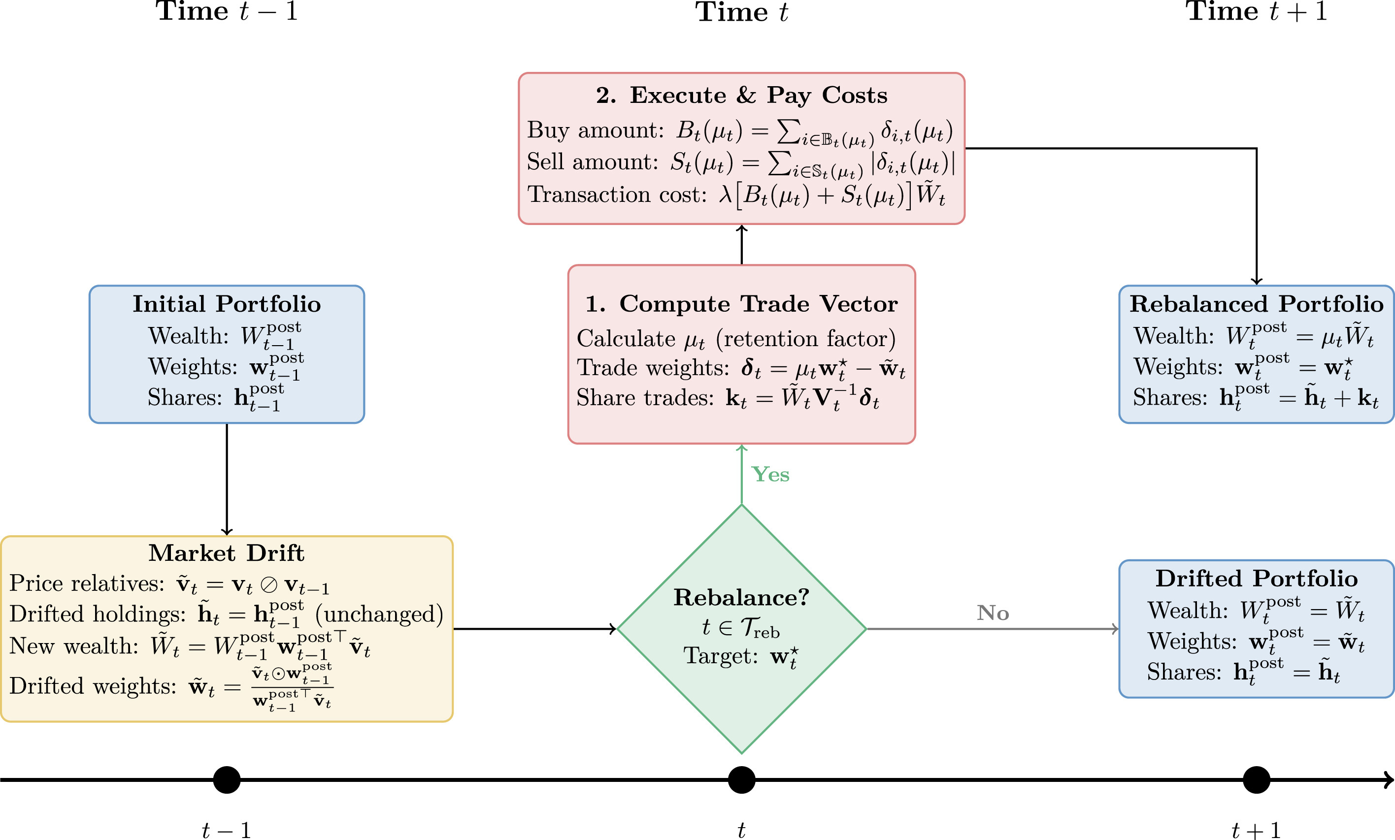
Price Drift and Weight Evolution

Between rebalancing dates, portfolios experience passive drift due to price movements. Trading days are indexed \(t \in \{0, 1, \ldots, T\}\) with rebalancing permitted on the subset \(\mathcal{T}_{\text{reb}} \subseteq \{1, \ldots, T\}\). For \(N\) risky assets with prices forming the vector \(\mathbf{v}_t = (1, v_{1,t}, \ldots, v_{N,t})^\top \in \mathbb{R}^{N+1}_{++}\) (where asset 0 represents cash with \(v_{0,t} \equiv 1\)), we work with simple one-period returns:

Portfolio weights must lie in the \((N+1)\) probability simplex \(\Delta_{N+1}\). Starting from post-rebalance values \(W^{\text{post}}_{t-1}\) and \(\mathbf{w}^{\text{post}}_{t-1}\), the portfolio drifts to:

where \(\tilde{\mathbf{v}}_t = \mathbf{v}_t \oslash \mathbf{v}_{t-1}\) is the price-relative vector, \(\oslash\) denotes element-wise division, and \(\odot\) denotes element-wise multiplication. Share holdings remain unchanged during the drift period.

The Transaction Remainder Factor

At each rebalancing date \(t \in \mathcal{T}_{\text{reb}}\), the investor specifies a target portfolio \(\mathbf{w}^*_t \in \Delta_{N+1}\). We model transaction costs through a remainder factor \(\mu_t\), borrowed from the online-portfolio-selection literature [1,2,3]:

The quantity \(\mu_t\) represents the fraction of wealth retained after paying transaction costs. Equality at the lower bound occurs only in the extreme case of complete portfolio liquidation and reconstruction (when the current and target portfolios have no overlap in risky assets).

Computing the Wealth Retention Factor

The trade vector \(\boldsymbol{\delta}_t(\mu) = \mu \mathbf{w}^*_t - \tilde{\mathbf{w}}_t\) represents required weight changes. Partitioning risky assets into buy set \(\mathbb{B}_t(\mu) = \{i : \delta_{i,t}(\mu) > 0\}\) and sell set \(\mathbb{S}_t(\mu) = \{i : \delta_{i,t}(\mu) < 0\}\), the aggregate magnitudes are:

The cash balance constraint requires that cash before trading plus net proceeds equals cash after purchases. Following Guo et al. [2,3], we define the root-finding function:

where \(\boldsymbol{\delta}^{\text{nc}}_t\) denotes the non-cash (risky asset) components of the trade vector. Since \(g_t\) is piecewise linear and strictly decreasing, the unique root can be located exactly by sorting breakpoints at ratios \(z_i = \tilde{w}_{i,t}/w^*_{i,t}\) and scanning to find where \(g_t\) changes sign. This provides an exact, closed-form solution for transaction costs.

Over the full investment horizon, wealth decomposes into market returns and transaction costs:

---

ESG Screening Methodologies

In the absence of comprehensive EU Taxonomy data, portfolio managers operationalize ESG commitments using third-party ratings as primary measurement instruments. We examine three screening methods representing different implementation approaches:

Percentile Threshold Construction: Assets with ESG scores exceeding a specific percentile threshold \(p\) are selected, where \(p\) represents a desired proportion of the asset universe (e.g., top 20%).

Best-in-Class Construction: Assets are ranked by ESG scores in descending order and sequentially added until the average ESG score of the selected subset falls below a predefined threshold. While traditional best-in-class approaches screen within sectors, we apply this filter across the entire universe to maintain comparability and capture portfolio-level ESG characteristics.

Asset Threshold Construction: Assets are directly filtered based on a fixed ESG score threshold. Only assets meeting or exceeding this threshold are considered for allocation.

We implement thresholds at 70, 75, 80, and 85, where 70 corresponds approximately to MSCI's "A" rating or Refinitiv's "B+" [4,5]. As thresholds increase, screening becomes progressively stricter: fewer firms qualify under each provider's scoring system, and the remaining universe consists of increasingly higher-rated assets.

---

Allocation Strategies

Equal-Weighted Portfolio (EWP)

The EWP strategy serves as a methodological baseline for isolating the direct impact of ESG screening on portfolio dynamics. At each rebalancing date \(t \in \mathcal{T}_{\text{reb}}\), given eligible set \(\mathcal{E}_t\) and target cash weight \(w_{\text{cash}} \in [0,1)\):

This uniform weighting makes post-trade weights a deterministic function of the ESG-eligible set, allowing straightforward attribution of turnover and transaction costs to ESG screening itself rather than optimization choices.

Minimum-Variance Optimization (MV)

The MV strategy reveals how portfolio optimization adapts to ESG constraints. At each rebalancing date, we solve:

where \(\boldsymbol{\Sigma}^{\mathcal{E}}_t\) is the covariance matrix estimated using Ledoit-Wolf shrinkage [6] applied to returns of assets in \(\mathcal{E}_t\). By computing the covariance matrix using only eligible assets, we avoid numerical artifacts from including zero-variance cash in the estimation.

The MV framework illuminates whether ESG screening systematically excludes assets critical for risk minimization. If excluded assets have low correlations with the eligible universe, the constrained portfolio may exhibit higher volatility despite optimization. Additionally, MV's concentrated allocations amplify the impact of rating disagreements—different providers' scores can lead to entirely different dominant assets in the optimized portfolio.

---

Block Bootstrap Simulation

To generate statistically valid inference across multiple scenarios, we employ a block bootstrap methodology that preserves temporal dependencies in both asset returns and ESG scores. The procedure is applied separately for each ESG data provider (Refinitiv, Bloomberg, MSCI).

Optimal Block Length

The optimal block length \(\hat{l}_{\text{opt}}\) is determined using the method of Politis and White (2004) [7], refined by Patton et al. (2009) [8]:

where \(\hat{G}\) and \(\hat{D}\) are consistent estimators based on the autocovariance structure and spectral density at frequency zero. This balances the tradeoff between preserving autocorrelation structure (longer blocks) and generating sufficient bootstrap variability (shorter blocks).

Simulation Procedure

For each of \(M\) bootstrap replications:

1. Generate synthetic data pairs \((R^{(m)}, \text{ESG}^{(m)})\) using block bootstrap with geometric block lengths averaging \(\hat{l}_{\text{opt}}\). By resampling returns and ESG scores jointly in blocks, we preserve both temporal autocorrelation and cross-sectional dependencies.
2. Reconstruct price paths via \(v^{(m)}_{i,t} = v^{(m)}_{i,t-1}(1 + r^{(m)}_{i,t})\).
3. Align ESG scores with publication dates: The algorithm identifies historical update dates by detecting changes in the original ESG time series. Bootstrapped values are retained at these dates and forward-filled between them, producing adjusted scores \(\text{ESG}^{(m)}_{\text{adj}}\) that prevent look-ahead bias.
4. Simulate portfolio evolution for each strategy \(s \in \mathcal{S}\), where each strategy is defined by a triple \((s_{\text{ESG}}, s_{\text{Alloc}}, s_{\text{Param}})\) specifying the ESG filtering method, allocation approach (EWP or MV), and filter parameters. The simulation filters eligible assets based on ESG criteria, computes portfolio weights, and executes rebalancing trades under transaction costs \(\lambda\) at each \(t \in \mathcal{T}_{\text{reb}}\).
5. Extract performance measures \(\theta^{(m)}_s\) from each simulated portfolio path \(\mathcal{P}^{(m,s)} = \{W^{\text{post}}_t, \mathbf{h}^{\text{post}}_t, \mathbf{w}^{\text{post}}_t, \mu_t, TC_t\}_{t=0}^{T}\). The metric function \(\mathcal{M}\) can extract various outcomes including terminal wealth, cumulative transaction costs, Sharpe ratios, maximum drawdown, or turnover statistics.

The collection \(\{\theta^{(m)}_s\}_{s \in \mathcal{S}, m=1}^{M}\) forms our empirical distribution for statistical inference, enabling rigorous comparison of strategies across multiple performance dimensions.

---

Statistical Inference

With bootstrap distributions in hand, we need rigorous methods to determine whether observed differences between ESG-screened and benchmark portfolios are statistically meaningful. We employ a dual approach combining paired permutation tests with bootstrap percentile intervals.

Permutation Test

For each strategy \(s\) compared against benchmark \(b\), and for any performance metric of interest (terminal wealth, Sharpe ratio, transaction costs, etc.):

1. Form paired differences \(\delta^{(m)} = \theta^{(m)}_s - \theta^{(m)}_b\) across \(M\) replicates
2. Compute the sample mean \(\hat{\Delta}_s = \frac{1}{M} \sum_{m=1}^{M} \delta^{(m)}\)
3. Generate \(B\) permuted means by randomly flipping signs: \(\hat{\Delta}^{(r)}_s = \frac{1}{M} \sum_{m=1}^{M} \varepsilon^{(m)} \delta^{(m)}\) where \(\varepsilon^{(m)} \sim \{-1, +1\}\)
4. Compute p-value \(= \frac{1 + \#\{r : |\hat{\Delta}^{(r)}_s| \geq |\hat{\Delta}_s|\}}{B + 1}\)

This tests the null hypothesis that ESG screening has no effect on the metric of interest. The sign-flip permutation is valid because under the null, positive and negative differences are equally likely.

Bootstrap Confidence Intervals

For the same paired differences: draw \(R\) bootstrap resamples of size \(M\) with replacement, compute the mean for each resample, and extract the \(\alpha/2\) and \((1-\alpha/2)\) quantiles. This yields a \(100(1-\alpha)\%\) confidence interval for the true mean difference \(\Delta_s = \mathbb{E}[\theta_s - \theta_b]\). When the interval excludes zero, we have evidence of a statistically significant effect.

---

Implications of the Framework

This methodology enables several key insights for portfolio managers:

• Performance attribution: By running ESG-screened and unscreened portfolios through identical market scenarios, we can isolate the performance impact of sustainability constraints from general market movements. The bootstrap distribution reveals not just average effects but the full range of outcomes across market conditions.
• Cross-market consistency: By applying identical methodology across S&P 500, S&P 400, and STOXX 600, we can identify whether ESG effects are universal or vary by market capitalization, geography, or regulatory environment. The framework is readily extensible to other equity universes.
• Provider-dependent outcomes: Since MSCI, Bloomberg, and Refinitiv often disagree on ESG scores (as documented in our previous post), the eligible universe differs by provider, leading to systematically different portfolio compositions, risk exposures, and return profiles.
• Threshold sensitivity: Stricter ESG thresholds mechanically reduce the investable universe and increase turnover volume as more assets cross eligibility boundaries at each rebalancing date.
• Rebalancing frequency effects: Different rebalancing intervals (monthly, quarterly, etc.) interact with ESG rating update frequencies to produce varying cost profiles. More frequent rebalancing captures ESG changes faster but incurs higher cumulative transaction costs.
• Strategy interaction effects: MV portfolios experience turnover from two sources—ESG membership changes and covariance-driven weight adjustments—while EWP portfolios respond only to membership changes. This allows decomposition of ESG-specific effects from optimization-induced trading.

Conclusion

The methodology presented here provides a rigorous framework for quantifying the full impact of ESG integration in portfolio management—not just transaction costs, but performance outcomes across multiple dimensions. By combining exact transaction cost calculations, realistic ESG score dynamics, and robust statistical inference, we can measure what has previously been difficult to disentangle: how sustainability constraints affect returns, risk, and operational costs simultaneously.

The key innovation lies in the joint bootstrap of returns and ESG scores, which preserves the complex dependencies between market movements and rating dynamics. This allows us to assess whether observed performance differences are statistically robust or merely artifacts of specific market conditions.

References

Primary source: Alkan, D., Ayari, R., & Paraschiv, F. (2026). Green Fees: Sustainability Impacts on Portfolio Management. International Review of Financial Analysis.
[1] Jiang, Z., Xu, D., & Liang, J. (2017). A deep reinforcement learning framework for the financial portfolio management problem. arXiv:1706.10059.
[2] Guo, S., Gu, J.-W., & Ching, W.-K. (2021). Adaptive online portfolio selection with transaction costs. European Journal of Operational Research, 295(3), 1074-1086.
[3] Guo, S., Gu, J.-W., Fok, C. H., & Ching, W.-K. (2023). Online portfolio selection with state-dependent price estimators and transaction costs. European Journal of Operational Research, 311(1), 333-353.
[4] MSCI (2024). MSCI ESG Ratings Methodology.
[5] LSEG (2024). Environmental, Social and Governance Scores from LSEG.
[6] Ledoit, O., & Wolf, M. (2004). A well-conditioned estimator for large-dimensional covariance matrices. Journal of Multivariate Analysis, 88(2), 365-411.
[7] Politis, D. N., & White, H. (2004). Automatic block-length selection for the dependent bootstrap. Econometric Reviews, 23(1), 53-70.
[8] Patton, A., Politis, D. N., & White, H. (2009). Correction to "Automatic block-length selection for the dependent bootstrap". Econometric Reviews, 28(4), 372-375.
Disclaimer: This research blog and the linked paper are provided for informational purposes only and do not constitute investment advice. Past performance does not guarantee future results. All investments carry risk of loss.